Langevin Field-Theoretic Simulations (L-FTS) of Diblock Copolymers on GPUs


Related Publications

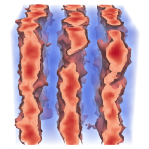
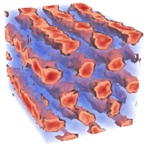
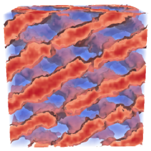
Fluctuation stabilization of the Fddd network phase in diblock, triblock, and starblock copolymer melts.
M. W. Matsen, T. M. Beardsley, and J. D. Willis
Self-consistent field theory has demonstrated that the homologous series of \((AB)_{M}\) starblock copolymers are promising architectures for the complex network Fddd phase. Nevertheless, it remains to be seen if the level of segregation will be sufficient to survive the fluctuations inevitably present in experiments. Here, we study the effect of fluctuations using field-theoretic simulations, which are uniquely capable of evaluating order-order phase transitions. This facilitates the calculation of complete fluctuation-corrected diagrams for the diblock \((M=1)\), symmetric triblock \((M=2)\), and nine-arm starblock \((M=9)\) architectures. Although fluctuations disorder the Fddd phase at weak segregations, they also stabilize the Fddd phase with respect to its ordered neighbors, which extends the Fddd region to higher segregation. Our results provide strong evidence that Fddd will remain stable in experiments on the side of the phase diagram where the outer \(A\) blocks of the star form the network domain. However, it is doubtful that Fddd will survive fluctuations on the other side where they form the matrix domain.

Fluctuation-corrected phase diagrams for diblock copolymer melts.
M. W. Matsen, T. M. Beardsley, and J. D. Willis
New developments in field-theoretic simulations (FTSs) are used to evaluate fluctuation corrections to the self-consistent field theory of diblock copolymer melts. Conventional simulations have been limited to the order-disorder transition (ODT), whereas FTSs allow us to evaluate complete phase diagrams for a series of invariant polymerization indices. The fluctuations stabilize the disordered phase, which shifts the ODT to higher segregation. Furthermore, they stabilize the network phases at the expense of the lamellar phase, which accounts for the presence of the Fddd phase in experiments. We hypothesize that this is due to an undulation entropy that favors curved interfaces.

Accounting for the ultraviolet divergence in field-theoretic simulations of block copolymer melts.
M. W. Matsen, T. M. Beardsley, and J. D. Willis
This study examines the ultraviolet (UV) divergence in field-theoretic simulations (FTSs) of block copolymer melts, which causes an unphysical dependence on the grid resolution, \(\Delta\), used to represent the fields. Our FTSs use the discrete Gaussian-chain model and a partial saddle-point approximation to enforce incompressibility. Previous work has demonstrated that the UV divergence can be accounted for by defining an effective interaction parameter, \( \chi = z_{\infty}\chi_{b} + c_{2}\chi_{b}^{2} + c_{3}\chi_{b}^{3} + \ldots \), in terms of the bare interaction parameter, \(\chi_{b}\), used in the FTSs, where the coefficients of the expansion are determined by a Morse calibration. However, the need to use different grid resolutions for different ordered phases generally restricts the calibration to the linear approximation, \(\chi \approx z_{\infty}\chi_{b}\), and prevents the calculation of order-order transitions. Here, we resolve these two issues by showing how the nonlinear calibration can be translated between different grids and how the UV divergence can be removed from free energy calculations. By doing so, we confirm previous observations from particle-based simulations. In particular, we show that the free energy closely matches self-consistent field theory (SCFT) predictions, even in the region where fluctuations disorder the periodic morphologies, and similarly, the periods of the ordered phases match SCFT predictions, provided the SCFT is evaluated with the nonlinear \(\chi\).

Well-tempered metadynamics applied to field-theoretic simulations of diblock copolymer melts.
T. M. Beardsley and M. W. Matsen
Well-tempered metadynamics (WTMD) is applied to field-theoretic simulations (FTS) to locate the order-disorder transition (ODT) in incompressible melts of diblock copolymer with an invariant polymerization index of \(\bar{N} = 10^{4}\). The polymers are modeled as discrete Gaussian chains with \(N = 90\) monomers, and the incompressibility is treated by a partial saddle-point approximation. Our implementation of WTMD proves effective at locating the ODT of the lamellar and cylindrical regions, but it has difficulty with that of the spherical and gyroid regions. In the latter two cases, our choice of order parameter cannot sufficiently distinguish the ordered and disordered states because of the similarity in microstructures. The gyroid phase has the added complication that it competes with a number of other morphologies, and thus, it might be beneficial to extend the WTMD to multiple order parameters. Nevertheless, when the method works, the ODT can be located with impressive accuracy (e.g., \(\Delta \chi N \sim 0.01\)).

Field-theoretic simulations for block copolymer melts using the partial saddle-point approximation.
M. W. Matsen and T. M. Beardsley
Field-theoretic simulations (FTS) provide an efficient technique for investigating fluctuation effects in block copolymer melts with numerous advantages over traditional particle-based simulations. For systems involving two components (i.e., \(A\) and \(B\)), the field-based Hamiltonian, \(H_{f}[W_{-}, W_{+}]\), depends on a composition field, \(W_{-}(r)\), that controls the segregation of the unlike components and a pressure field, \(W_{+}(r)\), that enforces incompressibility. This review introduces researchers to a promising variant of FTS, in which \(W_{-}(r)\) fluctuates while \(W_{+}(r)\) tracks its mean-field value. The method is described in detail for melts of \(AB\) diblock copolymer, covering its theoretical foundation through to its numerical implementation. We then illustrate its application for neat \(AB\) diblock copolymer melts, as well as ternary blends of \(AB\) diblock copolymer with its \(A-\) and \(B-\)type parent homopolymers. The review concludes by discussing the future outlook. To help researchers adopt the method, open-source code is provided that can be run on either central processing units (CPUs) or graphics processing units (GPUs).

Fluctuation correction for the order-disorder transition of diblock polymer melts.
T. M. Beardsley and M. W. Matsen
The order-disorder transition (ODT) of diblock copolymer melts is evaluated for an invariant polymerization index of \(\bar{N}=10^{4}\), using field-theoretic simulations (FTS) supplemented by a partial saddle-point approximation for incompressibility. For computational efficiency, the FTS are performed using the discrete Gaussian-chain model, and results are then mapped onto the continuous model using a linear approximation for the Flory-Huggins \(\chi\) parameter. Particular attention is paid to the complex phase window. Results are found to be consistent with the well-established understanding that the gyroid phase extends down to the ODT. Furthermore, our simulations are the first to predict that the Fddd phase survives fluctuation effects, consistent with experiments.

Computationally efficient field-theoretic simulations for block copolymer melts.
T. M. Beardsley, R. K. W. Spencer and M. W. Matsen
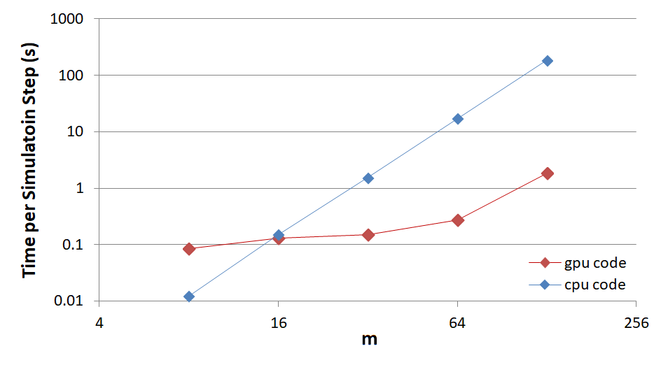
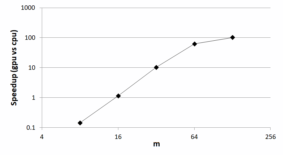
Field-theoretic simulations (FTS) provide fluctuation corrections to self-consistent field theory (SCFT) by simulating its field-theoretic Hamiltonian rather than applying the saddle-point approximation. Although FTS work well for ultrahigh molecular weights, they have struggled with experimentally relevant values. Here, we consider FTS for two-component (i.e., AB-type) melts, where the composition field fluctuates but the saddle-point approximation is still applied to the pressure field that enforces incompressibility. This results in real-valued fields, thereby allowing for conventional simulation methods. We discover that Langevin simulations are 1-2 orders of magnitude faster than previous Monte Carlo simulations, which permits us to accurately calculate the order-disorder transition of symmetric diblock copolymer melts at realistic molecular weights. This remarkable speedup will, likewise, facilitate FTS for more complicated block copolymer systems, which might otherwise be unfeasible with traditional particle-based simulations.

Calibration of the Flory-Huggins interaction parameter in field-theoretic simulations.
T. M. Beardsley and M. W. Matsen
Field-theoretic simulations (FTS) offer a versatile method of dealing with complicated block copolymer systems, but unfortunately they struggle to cope with the level of fluctuations typical of experiments. Although the main obstacle, an ultraviolet divergence, can be removed by renormalizing the Flory-Huggins \(\chi\) parameter, this only works for unrealistically large invariant polymerization indexes, \(\bar{N}\). Here, we circumvent the problem by applying the Morse calibration, where a nonlinear relationship between the bare \(\chi_{b}\) used in FTS and the effective \(\chi\) corresponding to the standard Gaussian-chain model is obtained by matching the disordered-state structure function, \(S(k)\), of symmetric diblock copolymers to renormalized one-loop predictions. This calibration brings the order-disorder transition obtained from FTS into agreement with the universal results of particle-based simulations for values of \(\bar{N}\) characteristic of the experiment. In the limit of weak interactions, the calibration reduces to a linear approximation, \(\chi \approx z_{\infty}\chi_{b}\), consistent with the previous renormalization of \(\chi\) for large \(\bar{N}\).

Project Motivations


Scientific Motivations


  1. Study diblock copolymer phase behaviour.
  2. Investigate realistic molecular weights.
  3. Identify equilibrium phases.
  4. Accurately detect order-disorder transitions.
  5. Produce diblock copolymer phase diagrams.
  6. Compare results to experiments, theory and other simulations.

Technical Motivations


  1. Field-based models (inc. L-FTS) are faster than particle simulations for intermediate/long chains.
  2. L-FTS can be adapted to study different architectures.
  3. Can take advantage of GPU hardware to maximise computational speed/efficiency.
  4. L-FTS avoids the instability that arises in complex langevin FTS.

Background Theory


Diblock Copolymers (DBCs)


A diblock copolymer consists of an A-block of \( N_{A} \) segments and a B-block of \( N_{B} \) segments (figure 1), joined together at one end to give a linear chain with \( N = N_{A} + N_{B} \) total segments and composition fraction \( f_{A} = N_{A}/N \).


Figure 1 - A diblock copolymer with \( N_{A} \) segments in the A-block and \( N_{B} \) segments in the B-block.


The strength of interactions between A and B segments is controlled by the Flory-Huggins parameter, \( \chi \), which is inversely related to temperature (i.e., low \( \chi \) corresponds to high temperature). When the A-B interactions in a melt of DBCs become sufficiently unfavourable (i.e., \( \chi \) becomes large enough) they microphase-separate, forming periodically ordered structures with domains on the nanometer scale. The equilibrium structures include the classical lamellar (L), cylindrical (C) and spherical (S) phases, as well as the complex gyroid (G) and Fddd phases (see figure 2).


Lamellar (L)
Cylinder(C)
Spherical (S)
Gyroid (G)
Fddd (Fddd)


Self-consistent Field Theory (SCFT)


Imagine looking at a single DBC in a melt. It has complicated interactions with all the other polymers in the system and capturing them all is a difficult mathematical and computational challenge.

SCFT addresses this problem by replacing the interactions that a polymer has with other chains by mean fields. The theory has been enormously successful in the study of DBCs, producing the famous equilibrium phase diagram shown in figure 3. It displays the various ordered phases, which are separated from the disordered phase by the order-disorder transition (ODT).

Figure 3 - The self-consistent field theory phase diagram for diblock copolymer melts.
Figure 4 - A schematic representation of the effect of fluctuations on the SCFT phase diagram in figure 3.


Limitations of SCFT


Unfortunately, the mean-field nature of SCFT means that it doesn't include the fluctuation effects that are inherent in real statistical systems. As a result, we are interested in fluctuation corrections to figure 3, which are controlled by the invariant polymerisation index, \( \bar{N} = a^{6}\rho_{0}^{2}N \), where \( \rho_{0} \) is the segment density and \( a \) is the statistical segment length.

SCFT corresponds to the case where \( \bar{N} = \infty \), with fluctuations increasing as \( \bar{N} \) is reduced. The main effects of fluctuations on the phase diagram in figure 3 are that the ODT gets shifted upward, and we get direct transitions between the disordered and ordered phases. For example, there will be a direct transition beween gyroid and disorder as indicated schematically in figure 4. We can see this behaviour in experiments...

Experimental Phase Diagrams


In 1994, Bates et. al. performed experiments to produce phase diagrams for three different DBC chemistries: PE-PEP (\( \bar{N}=27 \times 10^{3} \)), PEP-PEE (\( \bar{N}=3.4 \times 10^{3} \)) and PI-PS (\( \bar{N}=1.1 \times 10^{3} \)). Each of the phase diagrams exhibited the spherical, cylindrical and lamellar phases, but no gyroid or Fddd. There was, however, a region of another phase known as perforated lamellar in the region where SCFT predicts gyroid. Indeed, later experiments by Hajduk et. al. and Vigild et. al. showed that perforated lamellar is actually a long-lived metastable state that eventually converts to gyroid. Even more recent experiments by Wang et. al. and Takenaka et. al. have also confirmed the presence of Fddd on both sides of the phase diagram.

To reiterate, the significant differences in the phase diagrams of the experiments compared to the SCFT phase diagram are due to the effects of fluctuations near the ODT: the shifting up of the ODT and direct transitions between disorder and the ordered phases. It is these effects that we wish to capture in a field theory, and the next section shows how this problem is approached.

Polymer field theory


We start with a particle-base model (in our case a bead-spring model), which is fully specified by the polymer coordinates, \( {\bf r}_{\alpha,i} \), where \( \alpha = 1,2\ldots,n \) indexes the \( n \) polymers in the system and \( i = 1,2\ldots,N \) indexes the \( N \) monomers of a polymer. The particle-based hamiltonian takes the form $$\begin{eqnarray} \frac{H(\{ {\bf r}_{\alpha,i} \})}{k_{B}T} &=& \frac{3}{2a^{2}} \sum\limits_{\alpha=1}^{n} \sum\limits_{i=1}^{N-1} ( {\bf r}_{\alpha,i} - {\bf r}_{\alpha,i+1})^{2} \nonumber \\ &+& \rho_{0}\chi_{b} \int \hat{\phi}_{A} \hat{\phi}_{B} d{\bf r}, \nonumber \end{eqnarray}$$ where \(\hat{\phi}_{A}\) and \(\hat{\phi}_{B}\) are the concentrations of A and B monomers. The first term is the stretching energy arising from bonds between monomers, while the second is the energy from A-B interactions.

We then perform a mathematical transformation to give us a field-based model with hamiltonian $$\begin{eqnarray} \frac{H[W_{-},W_{+}]}{k_{B}T} &=& -n \ln Q[W_{-},W_{+}] \nonumber \\ &+& \rho_{0} \int \left( \frac{ W_{-}^{2}({\bf r})}{\chi_{b}} - W_{+}({\bf r}) \right) d{\bf r} \nonumber \end{eqnarray}$$ This field-based hamiltonian depends on two fields, \( W_{-}({\bf r}) \) and \( W_{+}({\bf r}) \), as well as the partition function of a single chain in these fields, \( Q \). The composition field, \( W_{-}({\bf r}) \), couples to the difference in A and B concentrations, while the pressure field, \( W_{+}({\bf r}) \), couples to the total concentration. It is important to note that \( W_{+}({\bf r}) \) is imaginary-valued, as this will become important as the theory progresses. In order to do calculations, we represent the fields on a mesh with grid spacing \( \Delta \), as shown in figure 6.


Figure 5 - A particle-based model of a diblock copolymer melt in a lamellar phase. The system is fully specified by the monomer coordinates, \( {\bf r}_{\alpha, i} \), where \( \alpha \) is the molecule index and \( i \) is the monomer index.
Figure 6 - A field-based model of a diblock copolymer melt in a lamellar phase. The system is fully specified by the real-valued composition field, \( W_{-}({\bf r}) \), and the imaginary-valued pressure field, \( W_{+}({\bf r}) \).


SCFT solution to polymer field theory


Self-consistent field theory obtains the fields by solving the following self-consistent equations: \[ \left( \frac{\mathcal{D}H}{\mathcal{D}W_{-}} \right) = 0, \quad \left( \frac{\mathcal{D}H}{\mathcal{D}W_{+}} \right) = 0, \] to obtain the saddle-point solutions of the fields \( w_{-} \) and \( w_{+} \). The free energy can then be approximated by \( F = H [w_{-}, w_{+}] \). However, since SCFT does not include fluctuation effects, we have to take a different approach...

Field-Theoretic Simulations (FTS)


The free energy of a system is given by \( F = - k_{B}T \ln (Z) \), where the partition function, \( Z \), is a sum over all possible microstates. For the field-based system, the partition function takes the form \[ Z \propto \int \exp \left( - \frac{H[W_{-}, W_{+}]}{k_{B}T} \right) \mathcal{D}W_{-} \mathcal{D}W_{+}. \] In field theoretic simulations, one attempts to simulate the full partition function directly, but there are still some issues to contend with.

Firstly, the \( W_{+} \) field is imaginary-valued, which gives us a complex-valued Boltmann weight (the exponential term). This means that it is not possible to use standard simulations techniques.

Secondly, since we represent the fields on a mesh, one might expect that as we reduce the grid spacing the results become more accurate. However, this is not the case due to the appearance of a UV divergence that must also be dealt with.

Complex Langevin FTS (CL-FTS)


One possible route to deal with the complex-valued Boltzmann weight is to perform complex Langevin FTS, where the fields evolve according to the equations: $$\begin{eqnarray} W_{-}({\bf r}; \tau + \delta \tau) &=& W_{-}({\bf r}; \tau) \nonumber \\ &-& \left( \frac{\mathcal{D}H}{\mathcal{D}W_{-}} \right) \delta \tau + \mathcal{N} (0, \sigma), \end{eqnarray}$$ and $$\begin{eqnarray} W_{+}({\bf r}; \tau + \delta \tau) &=& W_{+}({\bf r}; \tau) \nonumber \\ &-& \left( \frac{\mathcal{D}H}{\mathcal{D}W_{+}} \right) \delta \tau + i\mathcal{N} (0, \sigma), \end{eqnarray}$$ where \( \mathcal{N} (0,\sigma) \) is real-valued Gaussian noise with zero mean and standard deviation given by: \[ \sigma = \sqrt{\frac{2 \delta \tau}{\Delta^{3}\rho_{0}}}. \] However, there have been some issues with this approach discussed in the literature, including an instability in the complex-Langevin dynamics that makes it difficult to reduce \( \bar{N} \) to values typical of experiments. As a result, we take a different approach and use conventional Langevin FTS.

Partial Saddle-Point Approximation


We consider that the fluctuations in the pressure field, \( W_{+} \), are less important than those in the composition field, \( W_{-} \), and therefore approximate it by its saddle-point value, \( w_{+} \). The composition field remains fully fluctuating. The partial saddle point approximation results in the partition function: \[ Z \propto \int \exp \left( - \frac{H[W_{-}, w_{+}]}{k_{B}T} \right) \mathcal{D}W_{-}. \] The benefit to this approach is that since \( w_{+} \) is real-valued, this makes the exponential term \( Z \) real-valued and means we can use conventional simulation techniques. We choose Langevin field-theoretic simulations, as described in the next section.

Langevin FTS (L-FTS)


One of the advantages of L-FTS is that it does not suffer from the instability that makes CL-FTS troublesome. At each step of the simulation, the \( W_{-} \) field evolves according to: $$\begin{eqnarray} W_{-}({\bf r}; \tau + \delta \tau) &=& W_{-}({\bf r}; \tau) \nonumber \\ &-& \left( \frac{\mathcal{D}H}{\mathcal{D}W_{-}} \right) \delta \tau + \mathcal{N} (0, \sigma), \end{eqnarray}$$ and the saddle-point of \( W_{+} \) is calculated by solving the self-consistent equation: \[ \left( \frac{\mathcal{D}H}{\mathcal{D}W_{+}} \right) = 0. \] This is a different approach to SCFT where both fields are approximated by their saddle points, and to CL-FTS where both fields are fully fluctuating.

Dealing with the UV divergence


Now that we have dealt with the issue of the complex-valued Boltzmann weight arising in polymer field theory, we turn out attention back to the second problem: the UV divergence. Fortunately, polymer field theory is renormalisable. This means that the UV divergence can be removed by expressing all results in terms of an effective interaction paramter introduced by the Morse group. For the sake of simplicity we can use the linear expression, \[ \chi = z_{\infty} \chi_{b}. \] Here, \( z_{\infty} \) is the relative number of intermolecular contacts (the number of interactions a chain segment has with segments of other molecules), a parameter that can be calculated analytically. The bare interaction parameter, \( \chi_{b} \), comes directly from the L-FTS simulations. It is possible to go beyond the linear approximation and calculate higher-order contributions to \( \chi \) by performing a Morse calibration. However, the details are outside the scope of this brief introduction to the background theory.

L-FTS Simulation Code Requirements


Broad Simulation Requirements


  1. Read an input file defining simulation parameters and initial fields.
  2. Define a 3D mesh and assign initial fields to it.
  3. Use a Langevin update to propagate \( W_{-} \) forward in simulation time.
  4. Solve self-consistent equation to get the saddle point, \( w_{+} \), of the pressure field.
  5. Sample quantities such as the structure function, \( S(k) \), to facilitate detecting the ODT.
  6. Output the fields and averages so they can be visualised.
  7. Repeat steps 3 - 6.

Technical Simulation Requirements


  1. Use C/C++ (a low-level language) for fast execution.
  2. Identify code that would benefit from GPU parallelisation.
  3. Write custom CUDA kernels and execute them on the GPU.
  4. Benchmark parallel GPU code against serial CPU code.

GPU Parallelised Code Areas


Subsections


  1. Propagator Calculation
  2. Random Number Generation
  3. Langevin update of \( W_{-}({\bf r}) \)
  4. Partition Function, \( Q \)
  5. Composition and Pressure fields, \( \phi_{-}({\bf r}) \) and \( \phi_{+}({\bf r}) \)
  6. Anderson Mixing Algorithm


Propagator Calculation


Without going into the full mathematical details, the simulation needs to calculate the composition field, \( \phi_{-}({\bf r}) \), and total concentration field, \( \phi_{+}({\bf r}) \) multiple times in order to obtain \( w_{+} \) and update \( W_{-}({\bf r}) \) at each time step of the simulation.

However, \( \phi_{-}({\bf r}) \) and \( \phi_{+}({\bf r}) \) themselves necessitate calculation of forward and backward propagators given by the recursion relations: \[ q_{i+1}({\bf r}) = h_{i+1}({\bf r}) \int g(R) q_{i}({\bf r} - {\bf R}) d{\bf R}, \] \[ q_{i-1}^{\dagger}({\bf r}) = h_{i-1}({\bf r}) \int g(R) q_{i}^{\dagger}({\bf r} - {\bf R}) d{\bf R}, \] where \( i \) indexes the polymer segment, \( h_{i}({\bf r}) \) is related to the \( i^{th} \) monomer's field energy and \( g({\bf r}) \) is related to the stretching energy of polymer bonds (mathematical details).

Calculating the propagators from these recursion relations is the most costly part of the FTS simulations, which involves transforming to and from reciprocal space for \( N-1 \) of the monomers. Since there are both forward and backward propagators, this results in \( 2(N-1) \) fast Fourier transforms (FFTs) having to be performed every time \( \phi_{-}({\bf r}) \) and \( \phi_{+}({\bf r}) \) are calculated. Then, considering the fact that \( \phi_{-}({\bf r}) \) and \( \phi_{+}({\bf r}) \) have to be recalculated \( n_{AM} \) times at each time step of the simulation in order to solve the self-consistent equation for \( w_{+} \), the total number of FFTs per time step, \( 2(N-1)n_{AM} \), soon adds up.

In serial versions of the code, the transforms are done with the FFTW fast Fourier transform library. However, performing Fourier transforms is highly parallelisable so this portion of the code has been rewritten to take advantage of the CUDA cuFFT library on the GPU.

In order to maximise the benefits of performing FFTs on the GPU, there are a number of other considerations that must be taken into account.

Minimising Data Transfers

Firstly, it is important to minimise the number of data transfers between CPU (host) memory and GPU (device) memory due to the costly overhead associated with copying data between them. As a result, the code has been written such that all of the propagators are calculated on the GPU without any need for any memory to be copied to the host. This required that \( h_{i}({\bf r}) \) and \( g({\bf r}) \) were both calculated and accessible in GPU memory.

Batched FFTs

Secondly, performing an FFT using either the FFTW or cuFFT libraries requires setup of a "plan". A plan provides the FFT library with the information it needs to perform the FFT, such as whether to do a forward/backward transform and the size/dimensionality of the mesh. Two plans are required in this code: one for transforming from real to reciprocal space, the other for transforming in the reverse direction.

Since we must calculate recursion relations for forward and backward propagators, a sensible first approach would be the following:

  1. Set up plans for forward (\( \mathcal{F_{r \rightarrow k}} \)) and backward (\( \mathcal{F_{k \rightarrow r}} \)) Fourier transforms using the cufftPlan3d function of the cuFFT library.
  2. Set intial conditions, \( q_{i=1}({\bf r}) \) and \( q_{j=N}^{\dagger}({\bf r}) \), of the propagators.
  3. Calculate \( q_{i+1}({\bf r}) \), the forward propagator of monomer (\( i+1 \)), which involves transforms to and from reciprocal space via the \( \mathcal{F_{r \rightarrow k}} \) and \( \mathcal{F_{k \rightarrow r}} \) cuFFT plans.
  4. Calculate \( q_{i-1}^{\dagger}({\bf r}) \), the backward propagator of monomer (\( j-1 \)), which involves transforms to and from reciprocal space via the \( \mathcal{F_{r \rightarrow k}} \) and \( \mathcal{F_{k \rightarrow r}} \) cuFFT plans.
  5. Repeat steps 3-4 until \( q_{N}({\bf r}) \) and \( q_{1}^{\dagger}({\bf r}) \) have been calculated.

The above algorithm certainly works, but can be improved upon by considering that it may not be fully utilising the GPU.

To maximise throughput on the GPU (i.e., amount of calculations completed per unit time), we would ideally pass it enough work that all its threads are utilised in parallel. However, the FFTs being performed on the GPU in the algorithm above are limited by the simulation's 3D mesh size. For example, suppose there are \( 60000 \) threads available on the GPU, but we run a simulation that uses only \( 30^{3} = 27000 \) threads during a FFT. That means there are another \( 33000 \) threads not being used. The problem is that in spite of having plenty of work for the GPU to do, we have to calculate the propagators sequentially since \( q_{i+1}({\bf r}) \) depends on \( q_{i}({\bf r}) \) and \( q_{i-1}^{\dagger}({\bf r}) \) depends on \( q_{i}^{\dagger}({\bf r}) \) etc.

However, it should be noted that \( q({\bf r}) \) and \( q^{\dagger}({\bf r}) \) can be calculated independently of one another. I.e., the calculations for \( q({\bf r}) \) do not have any dependence on \( q^{\dagger}({\bf r}) \) and vice versa. Therefore, there would be no issue with calculating both of them at the same time if it were possible. Fortunately, the cuFFT library provides us with the cufftPlanMany() function, which allows us to set up a plan where multiple Fourier transforms can be batch processed. Put another way, cufftPlanMany() enables us to fast Fourier transform \( q({\bf r}) \) and \( q^{\dagger}({\bf r}) \) on the GPU at the same time, thereby double the amount of required threads and taking better advantage of the hardware for smaller systems.

The only complication in batch processing \( q({\bf r}) \) and \( q^{\dagger}({\bf r}) \) is that they must be in contigious memory, i.e., the arrays for \( q({\bf r}) \) and \( q^{\dagger}({\bf r}) \) must sit next to each other in the computer's memory. As a result, the arrays in this simulation have been set up in such a way that \( q_{1}({\bf r}) \) and \( q^{\dagger}_{N}({\bf r}) \) reside next to each other in memory, as do \( q_{2}({\bf r}) \) and \( q^{\dagger}_{N-1}({\bf r}) \) etc...

This reduces our algorithm to:

  1. Set up plans for forward (\( \mathcal{\hat{F}_{r \rightarrow k}} \)) and backward (\( \mathcal{\hat{F}_{k \rightarrow r}} \)) Fourier transforms using the cufftPlanMany() function of the cuFFT library.
  2. Set intial conditions, \( q_{i=1}({\bf r}) \) and \( q_{j=N}^{\dagger}({\bf r}) \), of the propagators.
  3. Calculate \( q_{i+1}({\bf r}) \), the forward propagator of monomer (\( i+1 \)), and \( q_{i-1}^{\dagger}({\bf r}) \), the backward propagator of monomer (\( j-1 \)), at the same time via transforms to and from reciprocal space with the (\( \mathcal{\hat{F}_{r \rightarrow k}} \)) and (\( \mathcal{\hat{F}_{k \rightarrow r}} \)) cufftPlanMany() plans
  4. Repeat step 3 until \( q_{N}({\bf r}) \) and \( q_{1}^{\dagger}({\bf r}) \) have been calculated.


Random Number Generation


At each "time" step in the simulation, Gaussian random noise is added to the \( W_{-}({\bf r}) \) field at every point on the underlying mesh. Since the total number of mesh point scales with the cube of the linear dimension (i.e., a cubic mesh with linear dimension \( m_{x} = 64 \) has a total of \( M = m_{x}^{3} = 262,144 \) points), there can be a significant number of random numbers and it makes sense to generate them in parallel on the GPU for speed. Furthermore, having the random numbers already accessible on the GPU means that we can subsequently use them to update \( W_{-}({\bf r}) \) on the GPU (see next section), rather than incurring the cost of copying the random numbers back to the CPU (host) and updating \( W_{-}({\bf r}) \) there.

To achieve GPU random number generation, I have taken advantage of the CUDA cuRand library. It has the advantage of the curandGenerateNormalDouble(...) function that generates normally distributed random numbers, rather than having to generate a uniform random distribution and manually transform it:

curandGenerateNormalDouble(
  curandGenerator_t generator,
  double *outputPtr, size_t n,
  double mean, double stddev
).


Langevin update of \( W_{-}({\bf r}) \)


Each Langevin update of the \( W_{-}({\bf r}) \) field is done with a Leimkuhler-Matthews algorithm (not detailed here), which was found by Vorselaars to be 10x quicker than predictor-corrector methods for the same accuracy.

Fourtunately, this algorithm can be applied to each mesh point independently so the code has been written to update \( W_{-}({\bf r}) \) on the GPU.


Partition Function, \( Q \)


The partition function, \( Q \), is required for the Langevin update of \( W_{-}({\bf r}) \), as well in calculating the composition field \( \phi_{-}({\bf r}) \), and the pressure field \( \phi_{+}({\bf r}) \). The simplest way to calculate \( Q \) is to integrate the forward propagator of the \( N^{th} \) monomer over all space: \[ Q = \int q_{N}({\bf r}) d{\bf r}, \] with the integral becoming a sum in the simulation code.

Since the propagator has already been computed on the GPU, it would be advantageous to calculate the sum there too, rather than copy \( q_{N}({\bf r}) \) back to the CPU (host) for summation. Doing so requires a reduction algorithm, so the reduce(...) function of the CUDA Thrust library is used. Thrust is a well-tested C++ template library for high-performance parallel computing, so its algorithms should be optimised and error free.


Composition and Pressure fields, \( \phi_{-}({\bf r}) \) and \( \phi_{+}({\bf r}) \)


Both \( \phi_{-}({\bf r}) \) and \( \phi_{+}({\bf r}) \) are calculated multiple times at each time step as part of obtaining the saddle point field, \( w_{-}({\bf r}) \). The composition field also forms part of the update to \( W_{-}({\bf r}) \) at the next time step. These two fields are given by the equations \[ \phi_{-}({\bf r}) = \frac{1}{NQ} \sum\limits_{i=1}^{N} \gamma_{i} \frac{q_{i}({\bf r}) q_{i}^{\dagger}({\bf r})}{ h_{i}({\bf r}) }, \] and \[ \phi_{+}({\bf r}) = \frac{1}{NQ} \sum\limits_{i=1}^{N} \frac{q_{i}({\bf r}) q_{i}^{\dagger}({\bf r})}{ h_{i}({\bf r}) }, \] where \( \gamma_{i} = +1 \) if monomer \( i \) is A-type, or -1 if it's B-type.

These are costly fields to evaluate serially, because the product \( q_{i}({\bf r}) q_{i}^{\dagger}({\bf r}) \) has to be evaluated \( N \) times for every mesh point. However, as discussed in the previous sections, all of the quantities required in the above equations are already available on the GPU. It is therefore straightforward to consider a single \( i \) and calculate \( q_{i}({\bf r}) q_{i}^{\dagger}({\bf r}) \) for all mesh points in parallel. By repeating this process for the \( i = 1 \ldots N \) monomers and summing the results, we vastly reduce the time taken to evaluate the fields.


Anderson Mixing Algorithm


The saddle point of the pressure field, \( w_{+}({\bf r}) \), is obtained by solving its self-consistent equation iteratively via an Anderson-mixing algorithm, as detailed by Stasiak and Matsen. It runs multiple passes until a desired error tolerance between the input and output fields is reached, signifying that the field equation for \( w_{+}({\bf r}) \) has been solved.

During each pass, several summations are performed over all mesh points, \( M \) - a large number for any reasonably-sized system. As a result, these have been adapted to be performed on the GPU via the transform_reduce(...) function of the CUDA Thrust library. The advantage of this particular function is that it also applies a transform to the input data before doing the summation, allowing the sum of squares and the sum of two multiplied arrays to be calculated as required in one call.

Furthermore, there are two parts of the algorithm that require updating each of the \( M \) elements in the \( w_{+}({\bf r}) \) array. The first is a "simple mix", which will be performed once on each pass. The second is an "Anderson mix", which gets called up to \( n_{h} \) times on each pass, where \( n_{h} \) is the maximum number of histories (constant). This, of course, can be costly to do multiple times in each of the multiple passes with the CPU, so I have written the kernels: simpleMix(...) and AMmix(...) to perform the mixing on the GPU, significanly speeding up the Anderson Mixing algorithm.

As an additional note, there is a also a matrix equation that is solved by LU decomposition once during each pass with the gsl_linalg_LU_decomp(...) and gsl_linalg_LU_solve(...) functions of the gsl library. While there is scope to parallelise this portion of the code using the cublas library, the matrix being solved measures \( n_{h} \times n_{h} \), where typically \( n_{h} \approx 10 \). Since this is a small matrix, any benefit in performing it on the GPU would be negligable compared to the other parts of the algorithm and not worth the additional complication.


GPU vs Serial Code Benchmarking


Since I have written both serial (cpu) and parallel (gpu) versions of this project code, they can now be run with identical input parameters (same workload) and compared to quantify the speedup.

Figure 7 - Average time taken per simulation step in the gpu and cpu L-FTS codes as a function of the linear mesh dimension, \( m \), for cubic grids with \( m_{\gamma} = m \) and \( \gamma = x,y,z \). Note the logarithmic scales on the x and y axes.
Figure 8 - Speedup of the gpu L-FTS code relative to the cpu version vs the linear mesh dimension, \( m \), for cubic grids with \( m_{\gamma} = m \) and \( \gamma = x,y,z \). Note the logarithmic scales on the x and y axes.

Simulation Setup


Simulations on the cpu and gpu are run in cubic boxes with linear mesh dimension \( m_{\gamma} = 8,16,32,64,128 \) and spacing between mesh points \(\Delta = 0.1095\), giving box sizes of \( L_{\gamma} = m_{\gamma}\Delta \) in each dimension \( \gamma = x,y,z \).

At each \( m_{\gamma} \), both simulations start from the same disordered configuration that was equilibrated below the order-disorder transition at \( \chi N = z_{\infty} \chi_{b} N = 9.0 \). Ideally, the same random number generator (RNG) and seed would be used so that the workload is exactly identical on the cpu and gpu, but since the RNGs are implemented with different libraries, this was not possible. However, the effect of the (very slight) fluctuations in workload between simulation steps should average out over the course of a short simulation and become negligable.

All gpu simulations run 1000 steps of equilibration and a further 1000 for statistics where the structure function was sampled at each time step. This is also the case for the cpu simulations with \( m_{\gamma} = 8,16 \) and \( 32 \). However, the larger cpu simulations are so time consuming that only (100, 100) and (50, 50) steps are used for (equilibration, statistics) respectively. Execution times are compared by calculating an average time per step.

Hardware


The cpu simulations were run on AMD Rome 7532 processors: 2.40 GHz, 256M cache L3.

The gpu simulations were run on a node with an AMD Milan 7413 processor: 2.65 GHz, 128M cache L3.
The gpu itself was an NVidia A100SXM4 with 40 GB memory.

While there is a slight difference in speed of the processors, this should become insignificant for the gpu code as relatively little of the hard work is being done by the cpu.

Results


Figure 7 displays the average execution time per Langevin step in the gpu code (red) vs the cpu code (blue) during the equilibration period. At the smallest mesh size, \( m_{\gamma} = 8 \), the cpu code is actually faster as the overhead involved in memory transfers to and from the gpu negates the benefits of performing the limited number of calculations in parallel. It would be rare for simulations to be run on such a small mesh, but it is an interesting extreme case regardless.

At \( m \approx 16 \) there is a crossover, beyond which the gpu code starts to become significantly faster for larger mesh sizes (red gpu line below the blue cpu line). Just how much faster is best demonstrated by figure 8, which plots the speedup gained by performing the simulations on the gpu relative to the cpu.

Speedup is defined as: \begin{equation} S_{T} = \frac{T_{\textrm{cpu}}}{T_{\textrm{gpu}}}, \end{equation} where \( T_{\textrm{cpu}} \) and \( T_{\textrm{gpu}} \) are the execution times for the cpu and gpu code for equivalent work.

Again, the smallest mesh size has a speedup of \( S_{T} \lt 1 \), indicating that the cpu code is faster in this single case. However, as the system size increases, the gpu code goes from being around \( 1.1\times \) faster at \( m = 16 \), to a massive \( 102\times \) faster for the largest mesh with \( m = 128 \). To put that into context, a \( 102\times \) speedup means that a simulation taking a week on the cpu can be completed by the gpu code in around 1 hour and 40 minutes!

Furthermore, on the logarithmic scales of the axes in figure 8, the data exhibits an approximately linear region between \( m = 8 \) to \( m = 64 \). This translates to a power law relationship \begin{equation} S_{T} \propto m^{\alpha}, \end{equation} with an exponent of \( \alpha \lesssim 3 \). Since the total number of mesh points in the system scales as the cube of the linear dimension, i.e., \( M = m^{3} \), the value of \( \alpha \lesssim 3 \) suggests that the code has been well parallelised, as the speedup is scaling with the total number of mesh points (amount of work).

However, by \( m = 128 \), the rate at which \( S_{T} \) increases in figure 8 has begun to slow. This suggests that the single gpu has become saturated by the large number of calculations and the \( \alpha \approx 3 \) scaling has been lost. Regaining the scaling could be done by splitting the work between multiple gpus, but realistically any published results have not necessitated grids of \( m > 64 \).


GPU L-FTS Code


The GPU code for this project can be found on my github page at: https://github.com/tmbeardsley/lfts_gpu/.

The corresponding CPU code is located at: https://github.com/tmbeardsley/lfts_cpu/