Lattice Monte Carlo Simulations of Diblock Copolymers with Parallel Tempering


Related Publications

Universality of block copolymer melts.
J. Glaser, P. Medapuram, T. M. Beardsley, M. W. Matsen, and D. C. Morse
Simulations of five different coarse-grained models of symmetric diblock copolymers are compared to demonstrate a universal (i.e., model-independent) dependence of the free energy and order-disorder transition (ODT) on the invariant degree of polymerization \(\bar{N}\). The actual values of \(\chi N\) at the ODT approach predictions of the Fredrickson-Helfand (FH) theory for \(\bar{N} \gtrsim 10^{4}\) but significantly exceed FH predictions at lower values characteristic of most experiments. The FH theory fails for modest \(\bar{N}\) because the competing phases become strongly segregated near the ODT, violating an underlying assumption of weak segregation.

Monte Carlo phase diagram for a polydisperse diblock copolymer melt.
T. M. Beardsley and M. W. Matsen
The phase diagram for an AB diblock copolymer melt with polydisperse A blocks and monodisperse B blocks is evaluated using lattice-based Monte Carlo simulations. Experiments on this system have shown that the A-block polydispersity shifts the order-order transitions (OOTs) toward higher A-monomer content, while the order-disorder transition (ODT) moves toward higher temperatures when the A blocks form the minority domains and lower temperatures when the A blocks form the matrix. Although self-consistent field theory (SCFT) correctly accounts for the change in the OOTs, it incorrectly predicts the ODT to shift toward higher temperatures at all diblock copolymer compositions. In contrast, our simulations predict the correct shifts for both the OOTs and the ODT. This implies that polydispersity amplifies the fluctuation-induced correction to the mean-field ODT, which we attribute to a reduction in packing frustration. Consistent with this explanation, polydispersity is found to enhance the stability of the perforated-lamellar phase.

Monte Carlo phase diagram for diblock copolymer melts.
T. M. Beardsley and M. W. Matsen
The phase diagram for diblock copolymer melts is evaluated from lattice-based Monte Carlo simulations using parallel tempering, improving upon earlier simulations that used sequential temperature scans. This new approach locates the order-disorder transition (ODT) far more accurately by the occurrence of a sharp spike in the heat capacity. The present study also performs a more thorough investigation of finite-size effects, which reveals that the gyroid (G) morphology spontaneously forms in place of the perforated-lamellar (PL) phase identified in the earlier study. Nevertheless, there still remains a small region where the PL phase appears to be stable. Interestingly, the lamellar (L) phase next to this region exhibits a small population of transient perforations, which may explain previous scattering experiments suggesting a modulated-lamellar (ML) phase.

Effects of polydispersity on the order-disorder transition of diblock copolymer melts.
T. M. Beardsley and M. W. Matsen
The effect of polydispersity on an AB diblock copolymer melt is investigated using lattice-based Monte Carlo simulations. We consider melts of symmetric composition, where the B blocks are monodisperse and the A blocks are polydisperse with a Schultz-Zimm distribution. In agreement with experiment and self-consistent field theory (SCFT), we find that polydispersity causes a significant increase in domain size. It also induces a transition from flat to curved interfaces, with the polydisperse blocks residing on the inside of the interfacial curvature. Most importantly, the simulations show a relatively small shift in the order-disorder transition (ODT) in agreement with experiment, whereas SCFT incorrectly predicts a sizable shift towards higher temperatures.

Background Science


Diblock Copolymers (DBCs)


A diblock copolymer consists of an A-block of \( N_{A} \) segments and a B-block of \( N_{B} \) segments (figure 1), joined together at one end to give a linear chain with \( N = N_{A} + N_{B} \) total segments and composition fraction \( f_{A} = N_{A}/N \).


Figure 1 - A diblock copolymer with \( N_{A} \) segments in the A-block and \( N_{B} \) segments in the B-block.


The strength of interactions between A and B segments is controlled by the Flory-Huggins parameter, \( \chi \), which is inversely related to temperature (i.e., low \( \chi \) corresponds to high temperature). When the A-B interactions in a melt of DBCs become sufficiently unfavourable (i.e., \( \chi \) becomes large enough) they microphase-separate, forming periodically ordered structures with domains on the nanometer scale. 
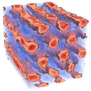
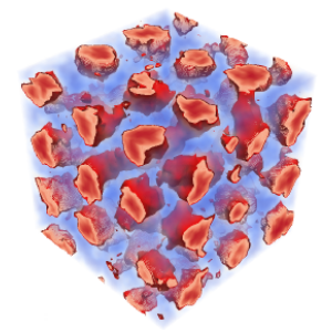
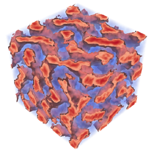
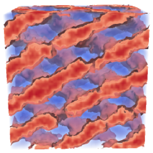
The equilibrium structures include the classical lamellar (L), cylindrical (C) and spherical (S) phases, as well as the complex gyroid (G) and Fddd phases (see figure 2).


Lamellar (L)
Cylinder(C)
Spherical (S)
Gyroid (G)
Fddd (Fddd)


Monodisperse vs Polydisperse DBCs


The typical model for studying diblock copolymer phase behaviour is the monodisperse melt, in which the \( n \) molecules of the system are identical with \(N_{A}\) monomers in the A-block and \(N_{B}\) monomers in the B-block. However, a melt of monodisperse molecules is difficult, time-consuming and expensive to produce in real experiments. There are cheaper chemical techniques to manufacture DBCs, but they result in relatively high levels of polydispersity.

In a polydisperse system, the molecules are no longer identical. There is a distribution of lengths in the A-block, the B-block or both, referred to as a molecular-weight distribution (MWD). Indeed, experimentally produced diblock copolymers are never truly monodisperse and always have at least a narrow MWD. The amount of polydispersity is measured by the polydispersity index, \( \mathcal{D} \), which is the ratio of the distribution's weight-average to number-average molecule length. For the A-block, this is can be expressed as \[ \mathcal{D}_{A} = \frac{(N_{A})_{w}}{(N_{A})_{n}} = \frac{\sum\limits_{N_{A}} N_{A}^{2} n_{N_{A}}}{n(N_{A})_{n}^{2}}, \] where \( n_{N_{A}} \) is the number of molecules in the distribution with an A-block of length \( N_{A} \) and \[ (N_{A})_{n} = \frac{1}{n} \sum\limits_{N_{A}} N_{A} n_{N_{A}}, \] is the number-average molecular weight of the A-block. The polydispersity index is \( \mathcal{D} = 1 \) for monodisperse molecules and increases as the MWD broadens.

One of the motivations of this project is to determine whether the novel self-assembly properties of diblock copolymers remain with the introduction of polydispersity, as well as how phase boundaries and properties such as domain size are affected by it.

Self-consistent Field Theory (SCFT)


Imagine looking a single DBC in a melt. It has complicated interactions with all the other polymers in the system and capturing them all is a difficult mathematical and computational challenge. SCFT addresses this problem by replacing the interactions that a polymer has with other chains by mean fields.

Monodisperse Phase Diagram
SCFT has been enormously successful in the study of DBCs, producing the famous equilibrium phase diagram for a monodisperse melt shown in figure 3. It displays the various ordered phases, which are separated from the disordered phase by the order-disorder transition (ODT). It is also worth noting that the phase diagram is symmetric about \( f_{A} = 1/2 \).

Figure 3 - The self-consistent field theory phase diagram for diblock copolymer melts.
Figure 4 - A schematic representation of the effect of fluctuations on the SCFT phase diagram in figure 3.


Polydisperse Phase Diagrams
In 2007, Matsen used SCFT to investigate the effects of A-block polydispersity (monodisperse B-block) on the DBC phase diagram. The MWD took the form of a Schultz-Zimm distribution, with the probability of a chain having \( N_{A} \) A-segments being \[ p(N_{A}) = \frac{ k^{k}N_{A}^{k-1} }{ (N_{A})_{n}^{k} \Gamma(k) } \exp \left( - \frac{kN_{A}}{(N_{A})_{n}} \right), \] where \( k = 1/(\mathcal{D}-1) \) and \( \Gamma(k) \) is the gamma function evaluated at \( k \).

Matsen found that in addition to skewing the phase diagram and inducing areas of macrophase separation (the phase diagrams can be seen in the abstract of the linked paper), the order-disorder transition (ODT) gets shifted down to lower values of \( \chi N \) at all compositions (\( f_{A} \)) as polydispersity increases. This effect is demonstrated schematically in figure 5.

Figure 5 - Schematic representation of how increasing A-block polydispersity shifts the ODT to lower values of \( \chi N \) at all compositions, \( f_{A} \), in SCFT.
Figure 6 - Schematic representation of how increasing A-block polydispersity in experiments shifts the ODT to lower values of \( \chi N \) at low values of \( f_{A} \), and to higher values at high \( f_{A} \).


Limitations of SCFT


Unfortunately, the mean-field nature of SCFT means that it doesn't include the fluctuation effects that are inherent in real statistical systems. As a result, we are interested in fluctuation corrections to figure 3, which are controlled by the invariant polymerisation index, \( \bar{N} = a^{6}\rho_{0}^{2}N \), where \( \rho_{0} \) is the segment density and \( a \) is the statistical segment length.

SCFT corresponds to the case where \( \bar{N} = \infty \), with fluctuations increasing as \( \bar{N} \) is reduced. The main effects of fluctuations on the monodisperse phase diagram in figure 3 are that the ODT gets shifted upward, and we get direct transitions between the disordered and ordered phases. For example, there will be a direct transition beween gyroid and disorder as indicated schematically in figure 4.

Experimental Phase Diagrams


Monodisperse Phase Diagram
In 1994, Bates et. al. performed experiments to produce monodisperse phase diagrams for three different DBC chemistries: PE-PEP (\( \bar{N}=27 \times 10^{3} \)), PEP-PEE (\( \bar{N}=3.4 \times 10^{3} \)) and PI-PS (\( \bar{N}=1.1 \times 10^{3} \)). Each of the phase diagrams exhibited the spherical, cylindrical and lamellar phases, but no gyroid or Fddd. There was, however, a region of another phase known as perforated lamellar in the region where SCFT predicts gyroid. Indeed, later experiments by Hajduk et. al. and Vigild et. al. showed that perforated lamellar is actually a long-lived metastable state that eventually converts to gyroid. Even more recent experiments by Wang et. al. and Takenaka et. al. have also confirmed the presence of Fddd on both sides of the phase diagram.

Whilst the experiments and SCFT phase diagrams exhibit a lot of good qualitative agreement, the significant differences are due to the effects of fluctuations near the ODT in the experiments: the shifting up of the ODT and direct transitions between disorder and the ordered phases.

Polydisperse Phase Diagram
In 2007, Lynd and Hillmyer studied PEP-PLA and PS-PI diblocks where the PLA and PS blocks were polydisperse and the other blocks had very narrow molecular-weight distributions. By fitting their data to a functional form for \( \chi \), the authors presented plots of the degree of segregation at the ODT, \( (\chi N)_{\textrm{ODT}} \), as a function of polydispersity at several diblock compositions, \( f \).

They observed that for \( f_{\textrm{PLA}} \lesssim 0.6 \), there was a decreasing trend in \( (\chi N)_{\textrm{ODT}} \) as polydispersity increased, while at slightly larger compositions \( (\chi N)_{\textrm{ODT}} \) increased with polydispersity.

The same trends were observed in the higher molecular-weight PS-PI system, where increasing polydispersity decreased \( (\chi N)_{\textrm{ODT}} \) for \( f_{\textrm{PS}} \lesssim 0.51 \), but led to an increasing trend for \( f_{\textrm{PS}} = 0.64 \).

Hence, in a diblock copolymer system where one block is polydisperse, the experiments broadly observe that increasing polydispersity in the minority block leads to a decrease in \( (\chi N)_{\textrm{ODT}} \), which is in qualitative agreement with the SCFT predictions. However, increasing polydispersity in the majority block increases \( (\chi N)_{\textrm{ODT}} \), the opposite of the downward shift predicted by SCFT. In a further departure from mean-field behaviour, experiments have only observed direct transitions between between disorder and the non-spherical ordered phases.

As was the case in the monodisperse system, the significant differences between the predictions of SCFT and experiments in the vicinity of the ODT are suspected to be due to fluctuations. It is therefore of interest to confirm whether this is the case with simulations.

Project Motivation


Scientific Motivation


  1. Determine whether fluctuations are responsible for the disagreement between theory and experiment regarding the polydispersity-induced shift of the order-disorder transition.
  2. Investigate whether the novel self-assembly properties of diblock copolymers persist with experimentally realistic levels of polydispersity.
  3. Identify equilibrium phases.
  4. Accurately detect order-disorder transitions.
  5. Produce diblock copolymer phase diagrams.
  6. Compare results to experiments, theory and other simulations.

Technical Motivation


  1. Universality of the system allows a lattice model to be used.
  2. Lattice-based models are faster than free-space models.
  3. The study of equiulibrium behaviour with Monte Carlo allows for fast, unphysical system updates.
  4. Parallel tempering can speed up simulations by annealing out defects and collecting data from multiple simulations simultaneously.

Simulation Code Requirements


Broad Simulation Requirements


  1. Read an input file defining simulation parameters and initial configuration.
  2. Define a 3D lattice and place initial configuration of molecules onto.
  3. Use a simulation algorithm that includes fluctuation effects.
  4. Sample quantities such as the structure function, \( S(k) \), energy, \( U \), and heat capacity, \( C_{V} \) to facilitate detecting the ODT.
  5. Periodically output the configuration and averages so they can be visualised.
  6. Go to step 1 (repeat).

Technical Simulation Requirements


  1. Use C/C++ (a low-level language) for fast execution.
  2. Identify code that would benefit from parallelisation.
  3. Take advantage of high performance computing on large clusters with MPI.
  4. Compare parallelised code to serial code.

Monte Carlo Methods (briefly)

In statistical physics, a system with fixed volume and number of particles in contact with a heat bath at a fixed temperature is referred to as a canonical ensemble. The partition function for a canonical ensemble, such as our diblock copolymer melt, is given by \[ Z = \sum\limits_{i} e^{- \beta E_{i}}, \] where \( E_{i} \) is the energy of microstate (specific configuration) \( i \) and \( \beta = 1/k_{B}T \). Using the partition function, it is possible to calculate the thermodynamic average of a system observable, \( A \), via: \[ \langle A \rangle = \frac{1}{Z} \sum\limits_{i} A_{i} e^{- \beta E_{i}}, \] where \( A_{i} \) is the value of observable \( A \) in state \( i \). For example, the thermodynamic average of the energy would be: \[ \langle E \rangle = \frac{1}{Z} \sum\limits_{i} E_{i} e^{- \beta E_{i}}. \] The problem is that the number of states in a system becomes so large that we can't possibly count them and calculate the partition function directly. This is where Monte Carlo simulations come in...

Monte Carlo simulations create what is known as a 'Markov chain', where the next state to be visited depends only on the current state. The parition function of the system is effectively sampled by visiting each system-state with the correct probability - less-likely states are visited fewer times that likely states. Samples of observables (such as energy) are taken periodically as the system evolves and subsequently averaged. The longer the simulations runs for (more states visited), the more accurately the Monte Carlo averages will approximate the true thermodynamic values. The algorithm used to update the system in this project is summarised as follows:

Monte Carlo Metropolis Algorithm


  1. The system begins in a state, \( i \), with energy \( U_{i} \).
  2. By performing one of the prescribed Monte Carlo moves, a small perturbation is made to the initial configuration in an attempt to move the system to state \( j \), with energy \( U_{j} \).
  3. The difference in energy, \( \Delta U = U_{j} - U{i} \), that would result from moving the system from state \( i \rightarrow j \) is calculated.
  4. If \( \Delta U \leq 0 \), then the accepted move from state \( i \rightarrow j \) is accepted, the system configuration is updated and we move to step 6.
  5. If \( \Delta U > 0 \), the system is attempting to adopt a higher energy state. In this case, generate a random number, \( R \). If \( R < \exp(-\Delta U / k_{B}T) \) then the move from \( i \rightarrow j \) is accepted and the system configuration updated. Otherwise, the system remains in the initial state, \( i \).
  6. Take samples contributing to Monte Carlo averages.
  7. Go to step 1 and repeat.

Benefits of Monte Carlo


There are many benefits to using the Monte Carlo method in this project, but the particularly significant ones are as follows:

Fluctuations are included
Because the Monte Carlo algorithm samples from the entire partition function of the system, this method inherently includes the effects of thermal fluctuations. This is in contrast to SCFT where the polymer interactions are approximated by mean-fields, thereby ignoring the fluctuation effects that are likely responsible for the differences between the theory and experiments (see section: 'Background Science').

Unphysical moves are permitted
The Monte Carlo algorithm is concerned with equilibrium behaviour and not the dynamics of how it gets from one state to another. It simply needs to sample all of the system's configurational states with the correct probabilities.

The desired property of the algorithm being able to reach every possible state is referred to as 'ergodicity'. The configuration space should be sampled as broadly and as quickly as possible, since it would be detrimental to our Monte Carlo averages to get stuck in a non-equilibrium state or to be cycling between only a few states. We attempt to make the system ergodic by a wise choice of Monte Carlo moves/updates, which do not have to obey physics in moving the system from state \( i \rightarrow j \). They can be anything we can think of that gets us to another valid state of the system. The snake, crank and flip moves used in this project are described in the section, 'Lattice Monte Carlo Simulation Details'.

Lattice Monte Carlo Simulation Details


Lattice Model Description


Each molecule in the system has \(N_{A}\) A-type monomers and \(N_{B}\) B-type molecules, such that there are \( N = N_{A} + N_{B} \) in total in a particular diblock. The monomers are placed on a lattice such that each lattice site may be vacant or occupied by a single monomer and bonded monomers must occupy nearest-neighbour sites. Although it would be more physically realistic to perform the simulations in free-space, a lattice construction is far less computationally expensive and allows for more Monte Carlo statistics to be collected per unit time.

The lattice is contructed by starting with an \( L \times L \times L \) cubic lattice with \( V_{c} = L^{3} \) sites and lattice constant, \( d \). The allowed lattice vectors can be described by \( {\bf r}_{i} = d(h,k,l) \), where \( i = 1,2,\ldots,L^{3} \) is the site number and \( h,k,l = 0,1,\ldots,L-1 \). By allowing only sites where \( h+k+l \) is even, a face-centred cubic (fcc) lattice with bond length \( b = \sqrt{2} d \) and \( V = V_{c}/2 = L^{3}/2 \) sites results. An fcc construction is used as its large coordination number (number of nearest-neighbours a particular site has) of \( z = 12 \) helps to alleviate the effects of the lattice. Periodic boundary conditions are implemented in all three dimensions to reduce the effects of the finite lattice size, requiring that \(L\) is an even number. The periodic boundary conditions mean that a molecule can travel off a face of the lattice and continue on the opposite face.

To allow the molecules room to move around and for the Monte Carlo algorithm to become efficient, the lattice is filled to a copolymer concentration of \( \phi_{c} \equiv nN/V \approx 0.8 \), where n is the total number of molecules in the system. Ideally, all lattice sites would be occupied, but this would make the Monte Carlo algorithm more complex, reducing its speed and the size of the systems that could be investigated.

Molecular interactions within the system occur only between nearest-neighbour A and B monomers. The strength of the interaction is given by \( \epsilon_{AB} \), from which a dimensionless Flory-Huggins parameter \[ \chi \equiv \frac{z\epsilon_{AB}}{k_{B}T} \] is defined.

At each Monte Carlo step (MCS), an attempt is made to change the system slightly by performing one of the available local moves. If the attempted move results in double occupancy of any lattice site, it is immediately rejected according to the Metropolis algorithm described in section 'Monte Carlo Methods'.

Local Monte Carlo Moves


Selection and implementation of the allowed Monte Carlo moves can have a large effect of the efficiency of the Monte Carlo algorithm. The moves should quickly update the system's configuration and efficiently sample its phase space. At each MCS, one of three moves: snake, crank or flip (figs 7a-c), is randomly attempted according to the predefined probabilities: \( P_{snake} = 0.45 \), \( P_{crank} = 0.45 \) and \( P_{flip} = 0.10 \).

Figure 7a - Snake move. The molecule attempts to move into a randomly picked site at its head or tail.
Figure 7b - Crank move. One of the non-end monomers attempts to move to a neighbouring site without changing its two bonded monomers.
Figure 7c - Flip move. The positions of monomers \( i \) and \( N-i \) are exchanged for the integers, \( s = 1 \) to \( N \).


Snake move
One of the system's \( 2n \) polymer-end monomers is randomly chosen, as well as one of its 12 nearest-neighbour sites. An attempt is made to move the chosen end-monomer into the selected site by shifting all the monomers comprising the molecule along the chain backbone, as in figure 7a. If the neighbouring site is occupied then the move is rejected, unless it's occupied by the monomer of the opposite chain end. In this case, all of the monomers shift around the loop without any double occupation occurring. The computational cost of the snake move is relatively low because the resulting energy change is calculated from only the contacts of the molecule's end and junction monomers.

Crank move
One of the system's \( n(N-2) \) non-end monomers is randomly chosen. An attempt is made to move the selected monomer into a neighbouring site while leaving the two monomers it is bonded to unchanged, as in figure 7b. Due to the fixed bond length, \( b \), required by the fcc lattice geometry, the possible bond angles and number of potential moves available to the selected monomer are \( 180^{\circ} \) (0), \( 120^{\circ} \) (1), \( 90^{\circ} \) (3) and \( 60^{\circ} \) (3). A \( 180^{\circ} \) bond angle leads to the move being immediately rejected since the monomer cannot be displaced. Otherwise, the number of neighbouring vacant sites that satisfy the bond angle are counted. If there are no vacant sites then the move is rejected. In all other cases, one of the vacant sites is chosen at random and the monomer is moved there. The crank move is computationally inexpensive since it only involves a single monomer.

Flip move
An attempt is made to flip a molecule randomly chosen from the system's \( n \) chains. This is achieved by swapping the positions of monomers \( i \) and (\( N-i \)) for all integers in \( i = 1 \) to \( N/2 \), as in figure 7c. Since the molecule already occupies the space it requires, it will never be rejected as a result of double site occupation. However, the flip move is computationally expensive compared the the snake and flip moves since the nearest neighbour contacts of each monomer in the chain must be counted.


Global Parallel Tempering Move


A parallel tempering Monte Carlo simulation consists of an extended ensemble of \( M \) replicas of a statistical system (the DBC melt), each at a different \( \chi \), where generally \( \chi_{1} < \chi_{2} < \ldots < \chi_{M} \). A simulation begins with each of the \( M \) replicas peforming one of the local snake, crank or flip Monte Carlo moves at each step. After \( n_{MC} \) steps have been performed, a global swap move is attempted between a pair of randomly selected neighbouring replicas. The randomly selected replicas are labelled \( c \) and \( d \) in figure 8, which outlines the PT algorithm. The global swap tries to exchange the configurations of replicas \( c \) and \( d \), which (in terms of our model's units) is accepted according to the probability \[ P_{c \leftrightarrow d} = \min \{ ~1, ~\exp( \Delta \chi_{cd} \Delta n_{AB,cd})/12) ~\}, \] where \[ \Delta \chi_{cd} = \chi_{c} - \chi_{d}, \] and \[ \Delta n_{AB,cd} = n_{AB,c} - n_{AB,d}. \] Here, \( n_{AB,c} \) is the number of AB-contacts in replica \( c \), running at \( \chi_{c} \).

Without going into the mathematical details (which can be seen in Earl and Deem's paper), we can interpret the PT acceptance criterion as always allowing a configuration swap if it lowers the energy of the extended ensemble of replicas. Otherwise, the probability of a swap occurring goes down exponentially as the energies of replicas \( c \) and \( d \) become more disparate.

Regardless of whether the PT move was accepted the cycle then repeats, with the replicas performing a further \( n_{MC} \) local moves followed by a PT swap etc.

Figure 8 - Global parallel tempering (PT) Monte Carlo move. A PT swap is attempted after every \( n_{MC} \) Monte Carlo moves, in which a neighbouring pair of replicas attempt to exchange their configurations. The move is accepted/rejected according to the PT acceptance probability detailed in the text.


Sequential Temperature Scans and Issues
We are interested in how various quantities such as energy, heat capacity and structure function vary with \( \chi \). Traditionally this is done with a sequential \( \chi \) scan, which starts with a simulation of \( \Lambda = \Lambda_{eq} + \Lambda_{st} \) (local) Monte Carlo steps run at \( \chi_{0} \). The first \( \Lambda_{eq} \) steps give the system time to reach equilibrium at the chosen \( \chi \), while the following \( \Lambda_{st} \) steps are to collect statistics for the Monte Carlo averages.

After the \( \Lambda \) steps have been completed, the interaction parameter is incremented by an amount \( \Delta \chi \), such that the next simulation in the sequential scan runs at \( \chi_{i} = \chi_{i-1} + \Delta \chi \). The final configuration of simulation \( i-1 \) also becomes the starting configuration of simulation \( i \), which then undergoes another \( \Lambda = \Lambda_{eq} + \Lambda_{st} \) (local) Monte Carlo steps, collecting a new, independent set of statistics. This procedure is repeated until we have covered the desired range of \( \chi \). The idea is that by starting the next simulation with final configuration of the previous one, the system should already be close to equilibrium.

The problem with this method is that it is easy for the system to fall into local free energy minima and become trapped in a non-equilibrium state. Imagine starting in a disordered state at low \( \chi \). We increase \( \chi \) until we cross the ODT into the ordered region where we know that the lamellar structure is the equilibrium phase. By the time the \( \Lambda_{eq} \) steps are complete, we would hope that a lamellar configuration has formed.

Unfortunately, as is often the case, we find that the system has fallen into what is referred to as a 'local free energy minimum'. This could represent, for example, a lamellar phase where two adjacent layers have become partially joined (i.e., the configuration has a defect). While the energy of configuration with a defect is lower than that of complete disorder (as we would hope since we are in the ordered region), it is not as low as the desired 'global free energy minimum' that corresponds to a defect-free lamellar phase - the true equilibrium state of the system. This non-equilibrium lamellar configuration with a defect may persist during the \( \Lambda_{st} \) steps during which statistics are collected, resulting in skewed Monte Carlo averages that are not representative of the true equilibrium phase.

The problem is that in order to break free of the local free energy minimum (remove the defect) the system must overcome an energy barrier, requiring the occurence of significant (unlikely) thermal fluctuations at the current \( \chi \). If it doesn't break free during the \( \Lambda \) Monte Carlo steps before which \( \chi \) is increased by a further \( \Delta \chi \), then there is the chance that the non-equilibrium configuration will persist for the remainder of the temperature scan. This is because increasing \( \chi \) reduces the thermal energy and fluctuations. As a result, all the data pertaining to the ordered phase region will not truly represent equilibrium behaviour.

The ways to combat this issue in a sequential \( \chi \) scan are to either reduce \( \Delta \chi \), increase \( \Lambda_{eq} \) or both. However, this can take a prohibitive amount of computation time, which is why we employ parallel tempering, the advantages of which are described below.


Figure 9 - Schematic representation of four parallel tempering replicas with \( \chi_{1} > \chi_{2} > \chi_{3} > \chi_{4} \), exploring the system's phase space. The high \( \chi \) (low temperature) replicas are confined to relatively small regions and are susceptible to becoming trapped in deep local free-energy minima. The low \( \chi \) (high temperature) replicas are able to explore the entire phase space more freely. (Diagram adapted from Earl and Deem).


Advantages of Parallel Tempering
Parallel tempering has a number advantages over the sequential temperature scans described in the previous section.

Firstly, the global swap move leads to more efficient sampling of phase space. As depicted in figure 9, the high \( \chi \) (low temperature) replicas of the extended parallel tempering ensemble are confined to relatively small regions of phase space, while the low \( \chi \) (high temperature) replicas are free to explore more readily.

Assuming that a configuration swap between two neighbouring replicas is accepted, the high \( \chi \) replica moves to the region of phase space that the lower \( \chi \) replica was exploring. This allows the high \( \chi \) replica to explore a different region of phase space, having broken free of the local minimum in which it was trapped. Conversely, the low \( \chi \) replica moves to the region that the high \( \chi \) replica was exploring (and may have been trapped in). However, the low \( \chi \) (high temperature) replica is not neccessarily confined to the local minimum due to its higher thermal energy and fluctuations, allowing it to break free and explore a wider region of phase space. In such a case, neither replica involved in the swap is now confined to the local minimum. In the simulations, this leads to improved sampling of phase space and corresponds to the parallel tempering scheme readily annealing out metastable states and defects from the system replicas. Configurations that contain defects get pushed towards the low \( \chi \) (high temperature) end of the extended ensemble, while the well-ordered configurations preferentially reside at the high \( \chi \) end. This is because the higher number of AB contacts in a configuration containing a defect becomes less costly to the extended ensemble if it is swapped to a lower \( \chi \) (higher temperature) replica and replaced with a more ordered configuration.

A further benefit of parallel tempering is the ease with which each replica can run on its own CPU in parallel on a computer cluster. The replicas must communicate when a swap is attempted, but this does not significantly affect the simulation speed as long as the swap frequency is not too high. Since statistics are then collected for a range of tempertures simultaneously with little increase in computational cost, many more Monte Carlo steps can be performed in each replica relative to an equivalent sequential temperature scan.

Figures 10a gives a schematic representation of how a typical parallel tempering Monte Carlo simulation is set up. A chain of replicas is set up at series of \( \chi \) values spanning the ODT.


Figure 10a - A series of parallel tempering replicas spanning the order-disorder transition of a diblock copolymer phase diagram. Each replica collects statistics at its \( \chi \) value and can swap configurations with its neighbours.
Figure 10b - A schematic representing the dependence of the number of AB-contacts, \( n_{AB} \), on the \( \chi \)-parameter for the first-order transition of a DBC melt. The sharp drop in \( n_{AB} \) signifies the ODT.


Typical Parallel Tempering Setup
Figure 10a gives a schematic representation of how a typical parallel tempering Monte Carlo simulation is set up. At a particular composition, \( f_{A} \), we begin with a series of replicas at \( \chi \) values spanning the ODT. The replicas start from an equilibrated athermal configuration (i.e., \( \chi = 0 \), so that AB contacts have no effect) generated from a serial code simulation. The difference in \( \chi \) between adjacent replicas must be small enough that there is a reasonable probability of swaps being accepted and this can require some adjustment. The choice of \( \chi \) values is informed by monitoring the swap acceptance rates between replicas during an initial parallel tempering test run. If the acceptance rate between neighbouring replicas at \( \chi_{i} \) and \( \chi_{k} \) is too low (\( \sim 20\% \)), we can add an additional replica at an intermediate value of \( \chi_{j} = (\chi_{i} + \chi_{k})/2 \). Swaps are attempted every \( 1000 \) Monte Carlo steps per monomer.

The ODT is expected to be a first-order transition, signified by a rapid drop in the number of AB-contacts/energy (see figure 10b) and a spike in the heat capacity of the system (in an infinite system the drop would be discontinuous). As a result, it is neccessary to have a higher density of replicas with a small \( \Delta \chi \) between them in the vicinity of the ODT, otherwise their energy distributions would not overlap and the acceptance rate would be vanishingly small.

Another factor affecting the swap acceptance rate is the size of the system, \( L \), since the number of AB-contacts, \( n_{AB} \) scales with \( L \). As a result, \( \Delta \chi \) will has to be reduced as \( L \) increases to maintain a reasonable swap acceptance rate.

Lattice Monte Carlo Code


Coming soon!